Naming: Copacabana and Miramar
To quickly identify each setup, we have named them. From now on, the arc lamps shall be known as “Copacabana” and “Miramar”.
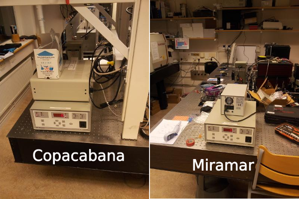
Figure 1: Where the Sun always shines…
Short note on history: Copacabana has a quite old bulb, and its intensity has clearly decreased over time. I re-adjusted the bulb and reflector of Copacabana today. Copacabana is equipped with a filter holder (attached to the lens tube) which holds a square AM1.5 filter.
Miramar has a new bulb, installed just a few days ago. Miramar does not come equipped with any attached filters.
Both lamps are set to operate at \(\SI{200}{\watt}\) (Miramar was previously set to \(\SI{250}{\watt}\) but was reset to the lower power limit after exhibiting a light fault error message and failing to ignite at the higher power).
Methods
Setup: total power using pyranometer
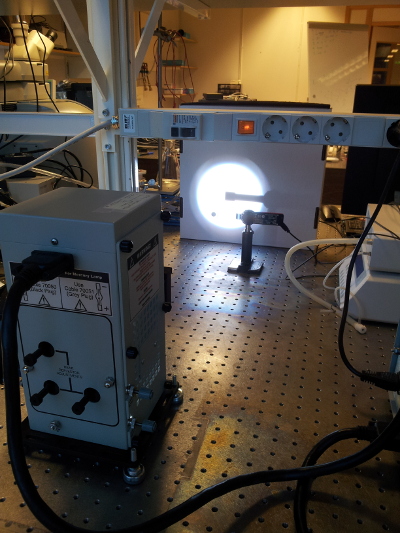
Figure 2: I measured the power output of Copacabana at varying distances.
Copacabana is equipped with a filter holder (on the lens tube) holding a square AM1.5 filter.
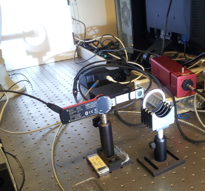
Figure 3: I measured the power output of Miramar at varying distances with an AM1.5 filter in the optical path.
I measured the power from the arc lamp at a range of distances using a Thorlabs PM160T power meter.
sensor.diameter <- 1.0 # cm
sensor.area <- pi * (0.5 * sensor.diameter)^2
area.corr.factor <- 1 / sensor.area
The sensor area is \(\SI{0.7854}{\square\cm}\), and consequently we need to multiply the values we read out with a factor 1.273 to get power densities (\(\si{\milli\watt\per\square\cm}\)).
It is also pertinent to mention how distances between lamp and sensor were measured.
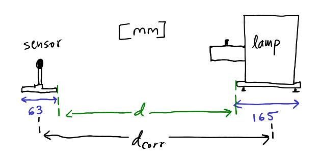
Figure 4: Sketch relating \(d\) and \(d_\text{corr}\) during measurement of total power
\[\begin{equation} d_\text{corr} = d + \frac{165}{2} + \frac{63}{2} = d + 114 \end{equation}\]
For practical reasons it was easier to measures the distances from one edge of each object to another, but for plotting and calculations I deemed it more correct to use centre-to-centre distance, which I termed \(d_\text{corr}\) (for corrected).
Setup: spectral profile of AM-filters
Measured the transmittance and absorbance of air-mass filters using the OceanOptics fibre-optic spectrometer.
AM filters:
- AM1.5 filter, square, usually mounted in arc lamp “Copacabana”
- AM1.5 filter, circular, loan from Andreas Mattsson
- AM0 filter, square (with small crack), loan from Andreas Mattsson
Note: according to Mattsson, his filters will produce AM1.5 when used in conjunction (both filters in the optical path).
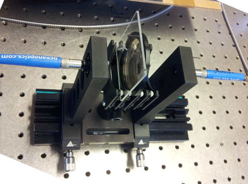
Figure 5: Measuring the spectral response of the air-mass filters.
Setup: spectral profile of ND-filters
Measured the transmittance of neutral density filters using the OceanOptics fibre-optic spectrometer.
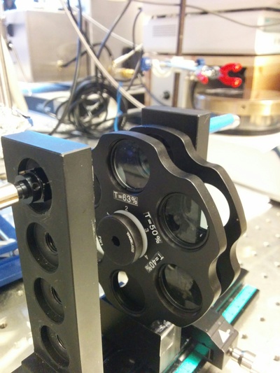
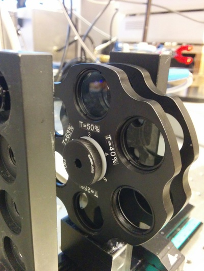
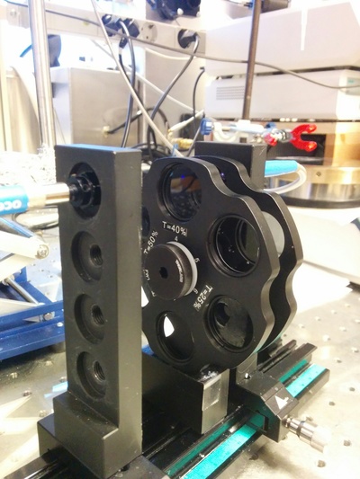
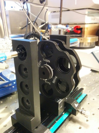
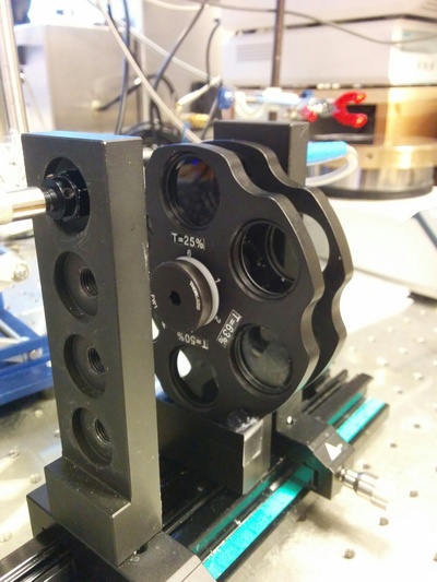
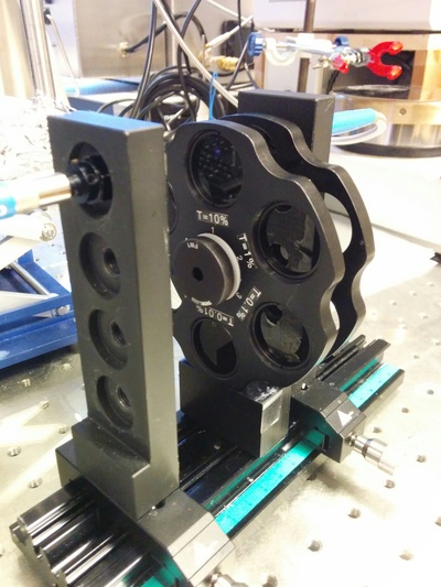
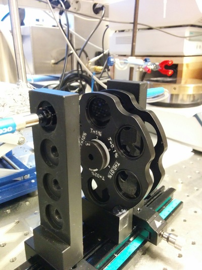
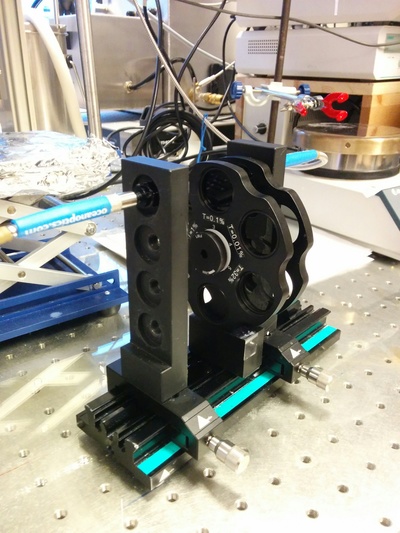
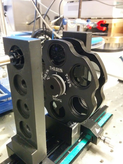
Photos of the ND-filter assembly. During each measurement the secondary ring was positioned so that an empty slot faced the optical beam. Combinations of filters were not measured (should be straight-forward to produce numerically if required).
Setup: spectral distribution of lamps
Characterised the spectra of both xenon arc lamps. The power of both lamps was high enough to saturate the spectrometer’s detector at all practical distances, so I did the spectral measurements with a 1% neutral density filter (that’s the wheel in the photos below) placed in front of the detector.
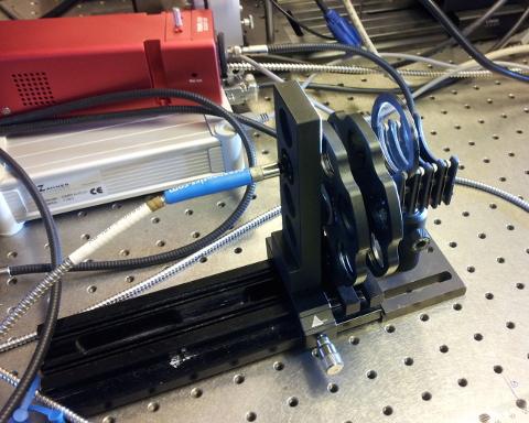
Figure 6: Measuring the spectral distribution of Miramar lamp.
The detector was at \(d=\SI{70}{\cm}\) (ie, \(d_\text{corr}=\SI{81.4}{\cm}\)), although that has little bearing on the results as we only want to compare spectral distributions of the lamps (power is compared via the pyranometer readings).
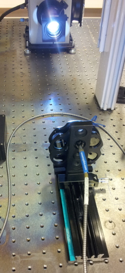
Figure 7: Measuring the spectral distribution of Copacabana lamp.
The detector was at \(d=\SI{60}{\cm}\) (ie, \(d_\text{corr}=\SI{71.4}{\cm}\)), although that has little bearing on the results as we only want to compare spectral distributions of the lamps (power is compared via the pyranometer readings).
Results
Total power of lamps
power <-
   cbind(lamp = "copacabana",
         read.csv(file = here::here("assets/copacabana-distance-vs-power.csv")))
power <-
   rbind(power,
         cbind(lamp = "miramar",
               read.csv(file = here::here("assets/miramar-distance-vs-power.csv"))))
power$corr.distance <- power$distance + 11.4 # cm
power$density <- round(power$power * area.corr.factor)
this.lamp <- "copacabana"
fit.copacabana <-
lm(density ~ logb(corr.distance, base = exp(1)),
data = subset(power, lamp == this.lamp))
x.copacabana <-
c(seq(1, 41),
subset(power, lamp = this.lamp)$corr.distance)
power.predicted.copacabana <-
predict(fit.copacabana,
newdata =
data.frame(corr.distance = x.copacabana))
power.calc.copacabana <-
data.frame(lamp = this.lamp,
distance = x.copacabana,
density = power.predicted.copacabana)this.lamp <- "miramar"
fit.miramar <-
lm(density ~ logb(corr.distance, base = exp(1)),
data = subset(power, lamp == this.lamp))
x.miramar <-
c(seq(1, 41),
subset(power, lamp = this.lamp)$corr.distance)
power.predicted.miramar <-
predict(fit.miramar,
newdata =
data.frame(corr.distance = x.miramar))
power.calc.miramar <-
data.frame(lamp = this.lamp,
distance = x.miramar,
density = power.predicted.miramar)# join power.calc dataframes
power.calc <-
rbind(power.calc.copacabana, power.calc.miramar)
Figure 8: Caption.
What is the distance at which each lamp yields total power corresponding to 1 Sun, ie \(\SI{100}{\milli\watt\per\square\cm}\)? Calculated by linear interpolation of the two points straddling the 100-mark for each curve (we’re not using the fitted exponential functions because I’m having some trouble applying the parameters).
Miramar’s “1 Sun” distance is \(\SI{57}{\cm}\) (centre-to-centre).
linfit.miramar <-
   approx(x = c(min(subset(subset(power, lamp == "miramar"), density <= 100)$corr.distance),
                max(subset(subset(power, lamp == "miramar"), density >= 100)$corr.distance)),
          y = c(min(subset(subset(power, lamp == "miramar"), density >= 100)$density),
                max(subset(subset(power, lamp == "miramar"), density <= 100)$density)),
          n = length(seq(max(subset(subset(power, lamp == "miramar"), density >= 100)$corr.distance),
                         min(subset(subset(power, lamp == "miramar"), density <= 100)$corr.distance),
                         by = 0.1)))
linfit.miramar$x[which(round(linfit.miramar$y) == 100)]
## [1] 55.5 55.6
And this is Copacabana’s “1 Sun” distance:
linfit.copacabana <-
   approx(x = c(min(subset(subset(power, lamp == "copacabana"), density <= 100)$corr.distance),
                max(subset(subset(power, lamp == "copacabana"), density >= 100)$corr.distance)),
          y = c(min(subset(subset(power, lamp == "copacabana"), density >= 100)$density),
                max(subset(subset(power, lamp == "copacabana"), density <= 100)$density)),
          n = length(seq(max(subset(subset(power, lamp == "copacabana"), density >= 100)$corr.distance),
                         min(subset(subset(power, lamp == "copacabana"), density <= 100)$corr.distance),
                         by = 0.1)))
linfit.copacabana$x[which(round(linfit.copacabana$y) == 100)]
## [1] 44.6
We’ll round that to \(\SI{45}{\cm}\).
Spectral response of air-mass filters
abs.files <-
   list.files(path = "/media/bay/taha/chepec/laboratory/OOHR2000/160423",
              pattern = "filter-A-.*\\.txt$",
              full.names = TRUE)
abs.data <-
   OO2df(datafile = abs.files[1], version = "1")
for (i in 2:length(abs.files)) {
   abs.data <-
      rbind(abs.data,
            OO2df(datafile = abs.files[i], version = "1"))
}
abs.data$technique <- "abs"
tra.files <-
list.files(path="/media/bay/taha/chepec/laboratory/OOHR2000/160423",
pattern = "filter-T-.*\\.txt$",
full.names = TRUE)
tra.data <-
OO2df(datafile = tra.files[1], version = "1")
for (i in 2:length(tra.files)) {
tra.data <-
rbind(tra.data,
OO2df(datafile = tra.files[i], version = "1"))
}
tra.data$technique <- "tra"# some clean-up to simplify plotting
tra.data <- subset(tra.data, (intensity <= 100) & (intensity >= 0))
abs.data <- subset(abs.data, intensity > -0.01)
# join abs and tra dataframes
exp.data <- rbind(abs.data, tra.data)
# trim noisy ends of spectra
exp.data <- subset(exp.data, (wavelength <= 1050) & (wavelength >= 260))
# rename the sampleids
exp.data$sampleid[which(exp.data$sampleid
%in% c("AM0-AM15-filter-A-AMattson",
"AM0-AM15-filter-T-AMattson"))] <-
"AM0+AM1.5"
exp.data$sampleid[which(exp.data$sampleid
%in% c("AM0-filter-A-AMattson", "AM0-filter-T-AMattson"))] <-
"AM0"
exp.data$sampleid[which(exp.data$sampleid
%in% c("AM15-filter-A-AMattson", "AM15-filter-T-AMattson"))] <-
"AM1.5-circ"
exp.data$sampleid[which(exp.data$sampleid
%in% c("AM15-filter-A-Copacabana", "AM15-filter-T-Copacabana"))] <-
"AM1.5-sq"
Figure 9: Caption.
Looking only at the \(\SIrange{300}{400}{\nm}\) range:

Figure 10: Absorbance and transmittance spectra of the AM filters (\(\SIrange{300}{400}{\nm}\)).
Using both the AM0 and AM1.5 (circular) filters in the optical path decrease transmittance markedly more than the AM1.5 (square) filter that we have used before.
Perhaps using only Mattson’s AM1.5 filter is the best compromise.
Spectral response of neutral density filters
nd.files <-
   list.files(path = "/media/bay/taha/chepec/laboratory/OOHR2000/171122-ND-filters",
              pattern = "\\.txt$",
              full.names = TRUE)
nd.data <- NULL
for (i in 1:length(nd.files)) {
   nd.data <-
      rbind(nd.data,
            OO2df(datafile = nd.files[i], version = "1"))
}
nd.data$technique <- "tra"
# some clean-up to simplify plotting
nd.data <-
nd.data %>%
filter(intensity <= 100 & intensity >= 0) %>%
# trim noisy ends of spectra
filter(wavelength >= 260 & wavelength <= 1050)
# a nicer label for the plot
nd.data$label <- paste0(sub("\\d{3}-ND-", "T = ", nd.data$sampleid), "%")
Figure 11: Spectral profile of each ND filter. Their absorbance is pretty constant within the range \(\SIrange{400}{800}{\nm}\). But below \(\SI{400}{\nm}\) their absorbance increases steeply.
Spectral distribution of lamps
# Copacabana with its "built-in" filter
lamp <-
   cbind(lamp = "Copacabana",
         filter = "AM1.5-sq",
         OO2df("/media/bay/taha/chepec/laboratory/OOHR2000/160423/Copacabana-lamp.txt",
               version = "1"))
# Miramar (which lacks built-in filter) while borrowing Copacabana's filter
lamp <-
   rbind(lamp,
         cbind(lamp = "Miramar",
               filter = "AM1.5-sq",
               OO2df("/media/bay/taha/chepec/laboratory/OOHR2000/160423/Miramar-lamp-AM15-Copacabana.txt",
                     version = "1")))
# Miramar with the circular AM1.5 filter
lamp <-
   rbind(lamp,
         cbind(lamp = "Miramar",
               filter = "AM1.5-circ",
               OO2df("/media/bay/taha/chepec/laboratory/OOHR2000/160423/Miramar-lamp-AM15-Mattson.txt",
                     version = "1")))
# Miramar with both of Mattson's filters (AM1.5 and AM0)
lamp <-
   rbind(lamp,
         cbind(lamp = "Miramar",
               filter = "AM0+AM1.5",
               OO2df("/media/bay/taha/chepec/laboratory/OOHR2000/160423/Miramar-lamp-AM15-AM0-Mattson.txt",
                     version = "1")))
# Finally, Miramar without any AM filters at all
lamp <-
   rbind(lamp,
         cbind(lamp = "Miramar",
               filter = "none",
               OO2df("/media/bay/taha/chepec/laboratory/OOHR2000/160423/Miramar-lamp.txt",
                     version = "1")))
Please keep in mind that the total power (area under the curve) in these spectra are not comparable between the two lamps since I did not bother placing the sensor at the same distance from the lamps. I was mainly interested in the spectral distribution.

Figure 12: Caption.

Figure 13: Spectral distribution of both lamps with the same AM1.5 filter in the optical path. Clearly, the spectral distribution is not affected by the age of the bulb (Copacabana ca 5 years old, Miramar brand new).
Actually, the main take-away from these measurements are that both lamps (new and old) produce the same spectral distribution, even though the stability and power of the new lamp is significantly better than the old.
Let’s have a closer look at short wavelengths:

Figure 14: Caption.
Keep in mind that the shown counts have not been zeroed, and that the zero-level is usually at approximately 650 counts.
Export experimental data to assets folder
# Note to self: use zip, not gzip, for compressing multiple files into one zip archive
system(paste("zip -j",
             here::here("assets/lnb-160423-filters.zip"),
             paste(list.files(pattern = "^.*-filter-.*\\.txt$",
                              full.names = TRUE,
                              "/media/bay/taha/chepec/laboratory/OOHR2000/160423"),
collapse = " ")))Session info
## Commit:  0057708e5b134d9aff01a590348209be7d467dc9
## Author:  taha@luxor <taha@chepec.se>
## When:    2021-03-07 00:02:33 GMT
##
##      Fixed the path to an asset
##
##      (the mistake was introduced when assets were bundled...)
##
## 1 file changed, 1 insertions, 1 deletions
## index.Rmd | -1 +1  in 1 hunk
## Untracked files:
##  Untracked:  index.Rmd.lock~
##
## Unstaged changes:
##  Modified:   index.Rmd
## R version 4.0.5 (2021-03-31)
## Platform: x86_64-pc-linux-gnu (64-bit)
## Running under: Ubuntu 18.04.6 LTS
##
## Matrix products: default
## BLAS:   /usr/lib/x86_64-linux-gnu/blas/libblas.so.3.7.1
## LAPACK: /usr/lib/x86_64-linux-gnu/lapack/liblapack.so.3.7.1
##
## locale:
##  [1] LC_CTYPE=C.UTF-8       LC_NUMERIC=C           LC_TIME=C.UTF-8
##  [4] LC_COLLATE=C.UTF-8     LC_MONETARY=C.UTF-8    LC_MESSAGES=C.UTF-8
##  [7] LC_PAPER=C.UTF-8       LC_NAME=C              LC_ADDRESS=C
## [10] LC_TELEPHONE=C         LC_MEASUREMENT=C.UTF-8 LC_IDENTIFICATION=C
##
## attached base packages:
## [1] grid      stats     graphics  grDevices utils     datasets  methods   base
##
## other attached packages:
##  [1] here_1.0.1             oceanoptics_0.0.0.9004 common_0.0.2
##  [4] git2r_0.29.0           directlabels_2021.1.13 ggrepel_0.9.1
##  [7] ggplot2_3.3.5          dplyr_1.0.8            magrittr_2.0.2
## [10] knitr_1.37
##
## loaded via a namespace (and not attached):
##  [1] Rcpp_1.0.8       pillar_1.7.0     bslib_0.3.1      compiler_4.0.5
##  [5] jquerylib_0.1.4  tools_4.0.5      digest_0.6.29    jsonlite_1.7.3
##  [9] evaluate_0.14    lifecycle_1.0.1  tibble_3.1.6     gtable_0.3.0
## [13] pkgconfig_2.0.3  rlang_1.0.1      cli_3.2.0        DBI_1.1.2
## [17] yaml_2.2.2       blogdown_1.7     xfun_0.29        fastmap_1.1.0
## [21] withr_2.4.3      stringr_1.4.0    generics_0.1.2   vctrs_0.3.8
## [25] sass_0.4.0       rprojroot_2.0.2  tidyselect_1.1.2 glue_1.6.1
## [29] R6_2.5.1         fansi_1.0.2      rmarkdown_2.11   bookdown_0.24
## [33] purrr_0.3.4      scales_1.1.1     ellipsis_0.3.2   htmltools_0.5.2
## [37] assertthat_0.2.1 colorspace_2.0-2 quadprog_1.5-8   utf8_1.2.2
## [41] stringi_1.7.6    munsell_0.5.0    crayon_1.5.0
## Linux 4.15.0-173-generic #182-Ubuntu SMP Fri Mar 18 15:53:46 UTC 2022 x86_64