Introduction
Scanning electron microscopy (SEM) is a powerful technique that is regularly used by chemists and other scientists to characterize an array of physical properties of a wide range of solid materials.
TIFF stands for Tagged Image File Format. Other than the image itself, the software can insert multiple tags with additional information, such as objective settings, acceleration voltage, stage position, etc. Timely recording of the experimental conditions is very important, so this feature of TIFF files is potentially very useful.
This post will demonstrate a method to extract TIFF tags from SEM micrographs using the R programming language. The method is particularly well-suited for SEM micrographs recorded using the SmartSEM® Operating Software1.
Unfortunately, the Zeiss SmartSEM® portal offers no download link to the software manual nor any other documentation on the software’s capabilities. And after perusing the SmartSEM® V05.06 and V05.04 software manuals, I found no description of the tags that the SEM software demonstrably attaches to the TIFF images.
But the manual does note that “images in BMP and JPEG format cannot be reloaded to the SmartSEM® user interface. Besides, it is not possible to save additional information with the image”. And in table 2.2 (“Available licenses”) of the manual, we learn of a “SmartSEM report generator” that “enables an Office 2007 add in ribbon that imports CZTIFF images and can read the tags so users can create reports”. But I have not tested the functionality of this report generator.
The only Zeiss-issued documentation related to TIFF files that we could find was a “technical information” sheet titled “The Tag Imaged File Format in the LSM” by Bernhard Reissner (1994) hosted on the research blog of former KTH PhD student Erland Lewin. The information in the document is interesting and sheds some light on the origins of attaching additional information in TIFF tags, but is severely outdated.
Notwithstanding the poor documentation offered by the SmartSEM® publisher, other microscopists have created scripts, plugins and software that can handle TIFF images to various degrees.
Most ambitious is probably tiffile.py by Christoph Gohlke (2014), a very well-documented Python script for reading and writing data from and to TIFF files. The script is geared towards handling the TIFF format in general, and does not collect the specific tags generated by the SmartSEM® software, but it could probably easily be expanded upon by someone with Python familiarity.
There is a MATLAB® function (should also work in Octave) that handles TIFF files, although it is mostly geared towards biophysics and LSM applications. tiffread.m v3.31 (licensed as GNU GPL v3) imports TIFF files into MATLAB/Octave. By Francois Nedelec of the Cell biology and Biophysics unit at EMBL (2013). Older versions of the same script are also found online [1, 2].
Then there is also a few ImageJ plugins that can read or dump TIFF tags,
and a SetScaleFromTiffTag ImageJ macro that (in conjunction with the TIFF tags ImageJ plugin above) can set the scale for SEM images taken with the Zeiss SmartSEM® software.
The TIFF format supports a few different kind of tags, specifically,
baseline tags are those that are listed as part of the core of TIFF, the essentials that all mainstream TIFF developers should support in their products, extension tags are those listed as part of TIFF features that may not be supported by all TIFF readers, private tags are, at least originally, allocated by Adobe for organizations that wish to store information meaningful only to that organization in a TIFF file. […], private IFD tags if one needs more than 10 private tags or so, the TIFF specification suggests that, rather then using a large amount of private tags, one should instead allocate a single private tag, define it as datatype IFD, and use it to point to a so called “private IFD”. In that private IFD, one can next use whatever tags one wants. These private IFD tags do not need to be properly registered with Adobe, they live in a namespace of their own, private to the particular type of IFD. [boldface added]
The above section is quoted from Joris van Damme who maintains a list of known tags and their descriptions and definitions.
SmartSEM® TIFF images
Below is a SEM micrograph recorded using Zeiss SmartSEM® V05.04.05.00 on a LEO1550 microscope (at the Ångström Microstructure Laboratory, Uppsala university).
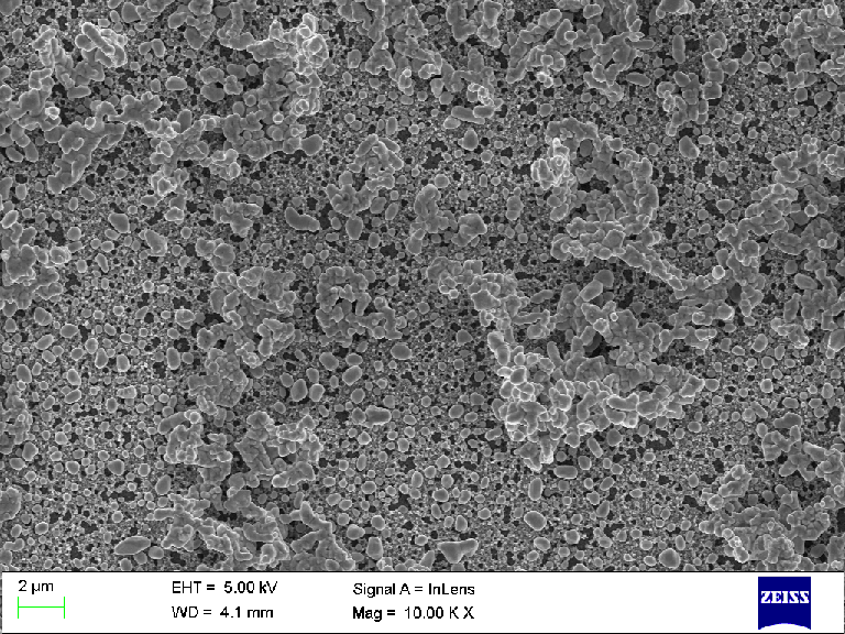
Short note: most TIFF editors honour the TIFF specification and discard tags/fields/IFD they do not understand. GIMP does too, and any edits made in GIMP on the original TIFF will cause all SmartSEM® tags to be discarded.
So if we want to read the tags that SmartSEM® so conveniently attaches to the TIFF images, we need to avoid editing the TIFF image or do our bidding before any edits.
To access the tags from the command line, we can use the TIFF tools collection, specifically, the tiffinfo utility. They are easily installed on GNU/Linux Debian-based systems:
sudo apt-get install libtiff-toolsThe extracted TIFF tags are just text (with some non-UTF8 characters, unfortunately), and we can easily write them to a file using piping.
tiffinfo micrograph.tif > tags.txt- TIFF tags extracted with
tiffinfofrom image taken with SmartSEM® V05.04.05.00 on LEO1550 scanning electron microscope - TIFF tags extracted with
tiffinfofrom image taken with SmartSEM® V05.06.00.00 on Merlin scanning electron microscope
For both software versions, tiffinfo reports that the tags are in a field with tag 34118 (0x8546), which indicates that SmartSEM® uses a so called private IFD tag to attach its array of parameters. It is also encouraging to see that the newer SmartSEM® version significantly expands the number of recorded parameters. Please note that we have removed the following parameters from the TIFF tag files above for privacy: SV_FILE_NAME, SV_USER_NAME, SV_OPERATOR, SV_USER_TEXT, SV_SERIAL_NUMBER, SV_IMAGE_PATH, SV_SAMPLE_ID, AP_DATE, AP_TIME.
We encourage the reader to inspect the SEM parameters stored in the TIFF tags, to get a feel for the scope of data that is recorded by the microscope.
Advantages of utilising the SEM parameters stored in TIFF tags
Although this particular SEM operating software (and probably others) record all pertinent instrument parameters into each TIFF image, I suspect that most users are not aware of this fact and still rely on taking notes in a lab notebook or similar, in addition to the few parameters that are usually embedded visually into the image itself (scalebar, magnification, acceleration voltage, and such, see example micrograph above).

The extracted TIFF tags incorporated into a LaTeX-generated micrograph report.
We have used a system where each micrograph was added to a SEM experiment report generated by LaTeX, with the a selection of the most relevant parameters included on the same page (see example above). It has worked well, but the report can of course not be generated until the SEM session is finished and all micrographs have been collected. As such, it is not a substitute for the lab notebook. A nice improvement would be to have the report page generated on a portable computer or tablet immediately after the image is saved by the microscope, and even better would be if the tablet or similar would allow the user to scribble notes on that generated report page. But I guess that is what an electronic lab notebook system is for…
Exploring the SEM dataset
if (!file.exists(here::here("assets/tiffiles.rda"))) {
   tif <- # all laboratory SEM TIFF files
      data.frame(files =
                    system("find /media/bay/taha/chepec/laboratory/SEM -type f -exec ls {} \\; | grep .tif",
                           intern = TRUE))
   tif$files <- sub("tif$", "txt", tif$files)
   # drop any textfile that does not exist (check for the sake of completeness)
   tif$files <- tif$files[file.exists(tif$files)]
   save(tif, file = here::here("assets/tiffiles.rda"))
} else {
   load(here::here("assets/tiffiles.rda"))
}
if (!file.exists(here::here("assets/tags.rda"))) {
   tags <- tiffalltags2df(tif$files[1])
   for (i in 2:dim(tif)[1]) {
      # this loop can take a while
      message(paste("Reading file", i, "of", dim(tif)[1]))
      tags <- rbind(tags, tiffalltags2df(tif$files[i]))
      }
   save(tags, file = here::here("assets/tags.rda"))
} else {
   load(here::here("assets/tags.rda"))
}
Our dataset consists of 927 SEM micrographs, recorded from 2011 to 2014. 672 micrographs were recorded using the LEO1550 microscope, and 255 micrographs were recorded using the Merlin microscope.
We will start this exploration by looking at the brightness vs contrast setting for all SEM micrographs. Since the majority of all SEM experiments were performed on similar samples (solid metal oxides of similar composition and morphology), we can assume that there should be a “sweet spot” of B and C values that the operator keeps repeating for best results. Also, we know from looking at the Auto BC parameter that BC was set manually for 96.9% of all micrographs.
Brightness vs. contrast using two different microscopes. The same data plotted against date shows that there is also an apparent improvement in operator proficiency over time.
Other than clear evidence of the hypothesized “sweet spot”, there is also an observable difference in B and C value clustering between the different microscopes. Although that could also be attributed to improved operator proficiency.
Here is another plot that highlights operator behaviour when recording micrographs. Number of micrographs consistently drop off with increasing magnification, with a few notable peaks at 35k and 90k.
Magnification of all recorded SEM micrographs. Low magnifications quite reasonable dominate the total number of recorded micrographs (every sample is explored at low magnification before zooming in).
And finally, a plot that explores the instruments more than the operator.
Pixel size vs. magnification. The difference between the two microscopes is interesting. Is it real, or just the result of different calibration?
Conclusion
If your scanning electron microscope uses Zeiss SmartSEM® software, you can take advantage of the fact that each TIFF image contains all the instrument parameters. In this post we have shown how those TIFF tags can be retrieved and saved using the R programming. We then used the aggregated TIFF tags from more than 900 of our own SEM images to investigate the relationship between a few parameters.
With the inclusion of what appears to be all instrument parameters in the SEM TIFF file, Zeiss has managed to set a good and bad example simultaneously. Good because it uses an established and open format, bad because the documentation is sorely lacking. Still, let’s hope that more scientific instrument makers emulate Zeiss’ example and attach the full set of instrument parameters to each output file, or at least make it optional.
If you liked this post and would like to see more like it, comment or contact me.
sessionInfo()
sessionInfo()
## R version 4.0.5 (2021-03-31)
## Platform: x86_64-pc-linux-gnu (64-bit)
## Running under: Ubuntu 18.04.6 LTS
##
## Matrix products: default
## BLAS:   /usr/lib/x86_64-linux-gnu/blas/libblas.so.3.7.1
## LAPACK: /usr/lib/x86_64-linux-gnu/lapack/liblapack.so.3.7.1
##
## locale:
##  [1] LC_CTYPE=C.UTF-8       LC_NUMERIC=C           LC_TIME=C.UTF-8
##  [4] LC_COLLATE=C.UTF-8     LC_MONETARY=C.UTF-8    LC_MESSAGES=C.UTF-8
##  [7] LC_PAPER=C.UTF-8       LC_NAME=C              LC_ADDRESS=C
## [10] LC_TELEPHONE=C         LC_MEASUREMENT=C.UTF-8 LC_IDENTIFICATION=C
##
## attached base packages:
## [1] stats     graphics  grDevices utils     datasets  methods   base
##
## other attached packages:
## [1] common_0.0.2   plotly_4.10.0  reshape2_1.4.4 ggplot2_3.3.5  knitr_1.37
##
## loaded via a namespace (and not attached):
##  [1] tidyselect_1.1.2  xfun_0.29         bslib_0.3.1       purrr_0.3.4
##  [5] colorspace_2.0-2  vctrs_0.3.8       generics_0.1.2    htmltools_0.5.2
##  [9] viridisLite_0.4.0 yaml_2.2.2        utf8_1.2.2        rlang_1.0.1
## [13] jquerylib_0.1.4   pillar_1.7.0      glue_1.6.1        withr_2.4.3
## [17] DBI_1.1.2         lifecycle_1.0.1   plyr_1.8.6        stringr_1.4.0
## [21] munsell_0.5.0     blogdown_1.7      gtable_0.3.0      htmlwidgets_1.5.4
## [25] evaluate_0.14     fastmap_1.1.0     fansi_1.0.2       Rcpp_1.0.8
## [29] scales_1.1.1      jsonlite_1.7.3    digest_0.6.29     stringi_1.7.6
## [33] bookdown_0.24     dplyr_1.0.8       grid_4.0.5        cli_3.2.0
## [37] tools_4.0.5       magrittr_2.0.2    sass_0.4.0        lazyeval_0.2.2
## [41] tibble_3.1.6      crayon_1.5.0      tidyr_1.1.4       pkgconfig_2.0.3
## [45] ellipsis_0.3.2    data.table_1.14.2 assertthat_0.2.1  rmarkdown_2.11
## [49] httr_1.4.2        R6_2.5.1          compiler_4.0.5
SmartSEM® V05.06 Operating Software for Scanning Electron Microscopes by Carl Zeiss Microscopy GmbH. Software manual [pdf, 15 MB].↩︎